
Table of contents
1. Download test files
2. A brief example
3. Plotting
1. Download test files
2. A brief example
2.1. Select 5', 3' and
gene body regions (GenomeIntervals2BED.py)
2.2. Overlap reads and genomic regions
2.3. Calculate sliding profiles
2.2. Overlap reads and genomic regions
2.3. Calculate sliding profiles
3. Plotting
3.1. Plot correlation
between TSS and TES coverage
3.2. Plot histograms
3.3. The gmx file
3.4. Plot box plots
3.5. Plot sliding profiles
3.2. Plot histograms
3.3. The gmx file
3.4. Plot box plots
3.5. Plot sliding profiles
1. Download test files
Before getting started:You will need “testfiles” folder that is distributed along SeqGI software. To download SeqGI visit the Download section. The "testfiles" folder contains:
- BED files of K4me3 reads (chr1 only) obtained from published datasets (Mikkelsen et al., 2007) in ES and NP cells, named “K4me3_ESchr1_mm9.bed” and “K4me3_NPchr1_mm9.bed”
- A list of gene groups in the gmx file format, named “ExampleGroups.gmx”
- Genomic coordinates for
mouse (mm9) UCSC known genes obtained from UCSC database, named
“mm9_canonical_chr1.txt”
2. A brief example
As an example, we will use the K4me3 ChIP-Seq sample obtained in ES cells to calculate its overlap with a set of genes. We will be using three gene regions:
- TSS region defined as a 5kb window flanking each annotated transcription start site (TSS).
- TES region defined as a 1kb window flanking each annotated transcription end site (TES).
- Gene body region defined as the complete gene region from TSS to TES
2.1. Select 5', 3' and gene body regions (GenomeIntervals2BED.py)
First, we need to convert the custom mm9_canonical_chr1.txt into a BED file that can then be used by OGRe.py. Use GenomeIntervals2BED.py to convert genomic coordinates file mm9_canonical_chr1.txt into a bed file. See the user section on GenomeIntervals2BED usage for more details.| #create
the directory where you will be saving your results $ mkdir testrun #TSS window $ python SeqGI_V1.1/GenomeIntervals2BED.py -f testfiles/mm9_canonical_chr1.txt -c 2,3,4,5 --cID=1 --wstrand --window=TSS:-5000:5000 -o testrun/mm9_canonical_TSS.bed #TES window $ python SeqGI_V1.1/GenomeIntervals2BED.py -f testfiles/mm9_canonical_chr1.txt -c 2,3,4,5 --cID=1 --wstrand --window=TES:-5000:5000 -o testrun/mm9_canonical_TES.bed #Gene body window $ python SeqGI_V1.1/GenomeIntervals2BED.py -f testfiles/mm9_canonical_chr1.txt -c 2,3,4,5 --cID=1 -o testrun/mm9_canonical_Body.bed |
2.2. Overlap reads and genomic regions
To compute the overlap we will use the OGRe script. See the user section on OGRe usage for more details.| #TSS
window python SeqGI_V1.1/OGRe_V0.2.py -x mm9_canonical_TSS.bed -y testfiles/K4me3_ESchr1_mm9.bed --tx=bed --ty=bed --to=overlap --sx --sy -o testrun/ES_TSS_result.txt #TES window python SeqGI_V1.1/OGRe_V0.2.py -x mm9_canonical_TES.bed -y testfiles/K4me3_ESchr1_mm9.bed --tx=bed --ty=bed --to=overlap --sx --sy -o testrun/ES_TES_result.txt |
2.3.
Calculate sliding profiles
With SeqGI and OGRe you can also
calculate the read distribution across features. The distribution
profile is calculated by using a sliding window that scans each genomic
interval defined in feature-set X.
In this example we will use the same files as before, i.e., a set of genes and a set of ChIP-seq reads:
The GMX file is a tab delimited file that defines groups of genes/features. This file should contain the same IDs present in the BED and Genomic Interval files. In the GMX format each column represents a group of features/genes. This file format is very useful since it can store large amounts of information and be easily edited (e.g. using excel). An example of a gmx file is shown here.
In this example we will use the same files as before, i.e., a set of genes and a set of ChIP-seq reads:
| #TSS
window python SeqGI_V1.1/OGRe_V0.2.py -x testrun/mm9_canonical_TSS.bed -y testfiles/K4me3_ESchr1_mm9.bed --tx=bed --ty=bed --to=sliding --bins=10 --btype=nuc --sx --sy -o testrun/ES_TSS_result_sliding.txt #TES window python SeqGI_V1.1/OGRe_V0.2.py -x testrun/mm9_canonical_TES.bed -y testfiles/K4me3_ESchr1_mm9.bed --tx=bed --ty=bed --to=sliding --bins=10 --btype=nuc --sx --sy -o testrun/ES_TES_result_sliding.txt #Gene body python SeqGI_V1.1/OGRe_V0.2.py -x testrun/mm9_canonical_Body.bed -y testfiles/K4me3_ESchr1_mm9.bed --tx=bed --ty=bed --to=sliding --bins=1 --btype=perc --sx --sy -o testrun/ES_Body_result_sliding.txt |
3. Plotting
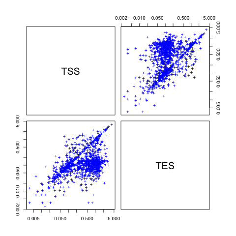
SeqGI output files can be used in R to plot. The script SeqGIplots.R is distributed within SeqGI and offers a collection of R functions that can be used for common graphical representations.3.1. Plot correlation between TSS and TES coverage
The plotCorrelation function allows you to plot pairwise comparison of the depth of coverage obtained for different sets of genomic intervals. In this example we will compare the scores obtained for TSS and TES windows:| #Enter
R $ R #Read in necessary files overlapname1 <- "Downloads/testrun/ES_TSS_result.txt" overlapname2 <- "Downloads/testrun/ES_TES_result.txt" #Load in R functions source("Downloads/SeqGI_V1.2/scripts/SeqGIplots.R") #Plot the pairwise correlation listoffilenames = list("TSS"=overlapname1, "TES"=overlapname2) plotCorrelation(listoffilenames, log="xy", col="blue") |
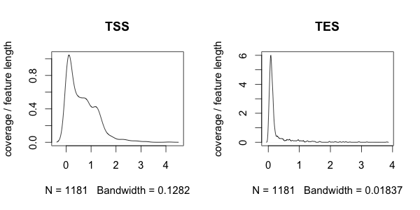
3.2. Plot histograms
The plothistogram function allows you to visualise the distribution of depth of coverage. In this example we will look at the distribution of depth of coverage in TSS and TES windows of genes:| #Enter
R $ R #Read in necessary files overlapname1 <- "Downloads/testrun/ES_TSS_result.txt" overlapname2 <- "Downloads/testrun/ES_TES_result.txt" #Load in R functions source("Downloads/SeqGI_V1.2/scripts/SeqGIplots.R") #Plot the histograms par(mfrow=c(1,2)) plothistogram(gmxname, overlapname1, main = "TSS") plothistogram(gmxname, overlapname2, main = "TES") |
3.3. The gmx file
The GMX file consists of a file format developed for the use with GSEA software (see GSEA wiki for details).The GMX file is a tab delimited file that defines groups of genes/features. This file should contain the same IDs present in the BED and Genomic Interval files. In the GMX format each column represents a group of features/genes. This file format is very useful since it can store large amounts of information and be easily edited (e.g. using excel). An example of a gmx file is shown here.
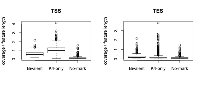
3.4. Plot box plots
The plotboxplot function allows you to compare the distribution of depth of coverage between subgroups of a given set of genomic intervals. To run this example we will make use of the gmx file which contains the lists of gene names. This file will be used to define each group of genes. For more details on the format of the gmx file please see the gmx section.| #Enter
R $ R #Read in necessary files gmxname <- "Downloads/testfiles/ExampleGroups.gmx" overlapname1 <- "Downloads/testrun/ES_TSS_result.txt" overlapname2 <- "Downloads/testrun/ES_TES_result.txt" #Load in R functions source("Downloads/SeqGI_V1.2/scripts/SeqGIplots.R") #Plot the boxplots par(mfrow=c(1,2)) plotboxplot(gmxname, overlapname1, main="TSS") plotboxplot(gmxname, overlapname2, main="TES") |
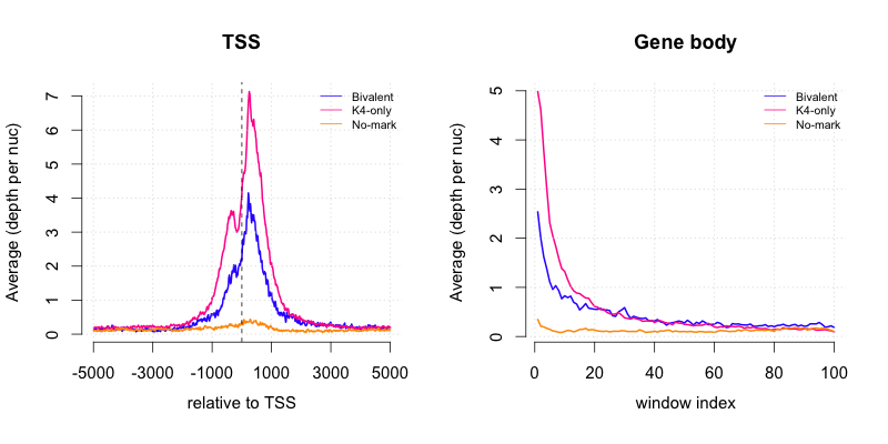
3.5. Plot sliding profiles
The plotsliding function allows you to compare the sliding window profiles between subgroups of a given set of genomic intervals. To run this example we will also make use of the gmx file which contains the lists of gene names.| #Enter
R $ R #Read in necessary files gmxname <- "Downloads/testfiles/ExampleGroups.gmx" slidingname1 <- "Downloads/testrun/ES_TSS_result_sliding.txt" slidingname2 <- "Downloads/testrun/ES_Body_result_sliding.txt" #Load in R functions source("Downloads/SeqGI_V1.2/scripts/SeqGIplots.R") #Plot the sliding profiles par(mfrow=c(1,2)) plotsliding(gmxname, slidingname1, wind=c("TSS",-5000,5000), main="TSS") plotsliding(gmxname, slidingname2, main="Gene body") |